 Mechanical
Music Digest™ Mechanical
Music Digest™ |
| You Are Not Logged In | Login/Get New Account |
|
Please Log In. Accounts are free!
Logged In users are granted additional features including a more current version of the Archives and a simplified process for submitting articles. |
|
|
MMD
|
Pushing and bouncing air
The good old topic of organ air supply surfaced again in the MMD Pipes Forum in 1999. At that time I learnt a lot from our experienced community about what devices you employ to get a stable air supply. Here is a brief review of these components and some of their properties described in acoustical engineering terms. Special attention is with the problem of regulation of transient loads, how to keep pressure constant across sudden changes in air demand. It is no cookbook on how to make a complete supply system - a prominent reason is the difficulty to specify what is required - but hopefully you may find some dimensioning guidelines from examples given. Basic formulas and diagrams are in SI units [6], but translations into traditional units are mostly shown in parallel. In an organ pipe the tone onset is very important and characteristic
and there are several factors to determine this onset. One is the pipe
itself as set up by the voicer. To keep a predictable pipe tone you must
also have control of how rapidly the playing valve opens and how well the
wind supply stands up to the increase in air demand when the pipe goes
on. Also any subsequent pressure changes will modulate the pipe tone, notably
when it sounds while other pipes go on or off, in particular in wide chords.
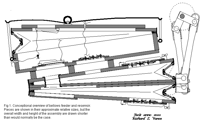
1. Sources 2. Reservoirs 3. Transmission trunks 4. Compensators 5. Bellows speed 6. Regulators 7. Complete feeder systems 8. References 9. Unit conversions and Air properties 1. SourcesClassical supply to bigger (church) organs up to the decades around 1900 was big weight loaded bellows. Each bellows had a lever to lift it and the organ blower(s) walked on these levers fast enough to maintain at least one of the bellows to be active. The regulation aspect here is that air pressure is then defined by those loading weights, not by the weight of the organ blower or how fast he works. This kind of source really does not belong in this section, but to the next of Reservoirs.Small as well as big street organs are usually powered from bellows,
agitated from a hand operated crankshaft. Modern modifications of these
most often include accumulator driven electric motors or gas engines to
drive them over a belt. Here are the outlines of a classical street organ
feeder [8]:
Without this tying up the feeder valves, the feeder would blow up the reservoir, were it not for the safety pallet. This one actually implements another principle of regulation, it is a spill regulator. Any surplus air is blown off, but in the same time you lose the energy you spent to pressurize it. Using spill regulation alone you have to provide full power to the crankshaft all the time. Apart from being wasteful this also makes noise, so spill regulation is mostly used for very small systems where simplicity and low cost may be important.
There are a few makers of specialized organ fans [5]. Beyond their load characteristic these are distinguished by silent operation due to careful balancing, solid housings, often cast, and a preference for sleeve bearings rather than ball bearings. Such fans have a noise level about 50 to 60 dBA and cost typically three times more than equivalent industrial fans which are 20 to 30 dB more noisy. The pneumatic power you supply to an organ is pressure times flow, W=PU. It is convenient to use SI units for P and U such that the power comes out in Watts without conversion factors. For instance, in the fan diagram P=1.1 kPa and U=200 m3/h=0.056 m3/s gives W=1100*0.056=61 Watts. Installed drive motor nominal power is normally several times bigger than this pneumatic power. And finally delivered sound power to the order of 1% of it. 2. ReservoirsThe reservoir obviously holds a spare quantity of pressurized air ready for immediate use, possibly to fill transient loads bigger than what is continuously available from the source. A main function however is to define a system pressure, which will be F=(total normal force on the reservoir lid) divided by A=(area of lid). Pressure P=F/A. Often the reservoir lid is also a sensing element in a regulating system.
The lid force may in stationary cases be exerted by weights (iron bars, stones, concrete blocks), now more often by springs, always so in portable applications. An easy way to estimate it is to start from the required pressure, expressed in terms of water column height. Multiply this height by the lid area - then you get a volume of water having the required weight.
The obvious part of the lid force is that from the weight or spring. A weight will give a constant force while a spring generally delivers a greater force the more the reservoir is filled. But there is also another force acting on the lid, namely from the bellows folds. With a sack reservoir this is essentially small and independent of lid position. But with a gusseted ribs reservoir this force will vary depending on filling degree.
The lower bellows is inward folded, between frames A and B, and here the vertical component on the ribs try to pull the frames together, they counteract the pressure on the lid which balances the weight or spring. This effect is most pronounced when the bellows are almost collapsed since the vertical component decreases with growing a as the lid lifts. The horizontal component works the opposite way, it grows with a, and it makes the ribs try to wedge the frames apart, it cooperates with the pressure on the lid. The total result is that when you fill a single, weight loaded inward folded reservoir the pressure decreases as you fill it. Contrarily, in the upper outward folded bellows between frames B and C, the rib forces change sign. So when you fill a single, weight loaded outward folded reservoir the pressure increases as you fill it. The specific feature of the illustrated double bellows design is to have these opposing actions to neutralize each other. But to make this work you must force frame B to be mid-way between A and C, effected by the pantograph mechanism D. This double bellows then keeps constant pressure, independent of filling degree, when compressed by a weight.
Accounting for those extra forces from the folding ribs, the relation between the external bellows compression force F and pressure P can be formulated as a bellows equation: F/P = A ± B*0.5*(sin(a)*tan(a)-cos(a)) [m2]where A is the lid area, B is folding rib area (one layer only, as seen in a top projection drawing of the bellows), and a is the opening angle of the folds. Plus sign for inward folds, minus for outward. An important special case is at a=45 degrees, ribs at right angles to each other. Then the complicated coefficient for B becomes zero and pressure equals the nominal P=F/A. 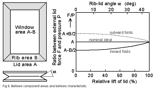
A reservoir is normally supplied from some power machinery and the forces involved are considerable. With an inward folded bellows there is a hazard inherent from the rise in the F/P characteristic shown in fig. 6. Keeping constant pressure, as angle grows you need a progressively greater force to balance it, indeed infinite force at a=90 deg. It is essential that you limit the angle to protect the bellows from such overload, otherwise it will be blown out and ripped apart. Usually you do that with a pallet safety valve on the lid, operated with a string or a finger toward some fixed structure, as exemplified in fig. 1. Normally you would allow a lid to rib angle a no more than about 45 degrees. With a spring loaded reservoir the spring force increases in proportion to the lid lift. Then the best is to use an inward folded reservoir. Ideally, for constant pressure, the force should then grow with a the same way as the complicated right hand expression. But we can reasonably well match this with a straight line. For given areas A and B, and pressure P, we may use for a rule of thumb that the spring force at full lift should be F(100%) = P*A, and with the bellows collapsed, F(0%) = P*(A - 0.6*B). That magic coefficient 0.6 is derived from the criterion that pressure around 20% lift should be the same as at 100%. Deviation from the ideal increases with B/A. Using B/A=0.5 as drawn in fig. 6, then pressure will be some 6% too high around 60% lift. For better precision you may reduce B, but that implies that the bellows volume capacity goes down in proportion.
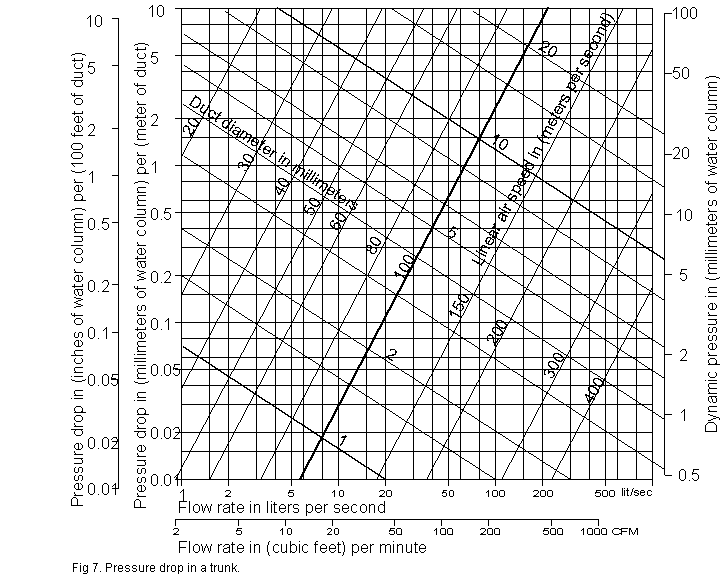
3. Transmission trunksThe air distribution trunks are a necessary evil and should obviously be kept as short, as wide, as straight, and as airtight as possible. Their consequences and countermeasures to those are the main topic of this article. The trunks are classically built from wood planks or boards. Nowadays metal or plastic tubing is often more convenient, e.g. tubes and joints with rubber gaskets as fabricated for sewage plumbing.3.1. Pressure losses in steady air transportWhen you steadily transport a volume flow U using a duct (the general technical term for a trunk) of length L and diameter D, then you will suffer a pressure drop P. This drop has two basic components, the viscous Pvisc and the kinetic Pkin.Pvisc is the result from the internal viscosity of air. This is the component generally talked about and it behaves well in the sense that is is directly proportional to the length of the trunk. The drop is larger as flow rate increases or the trunk is narrower. Computation is rather complicated as the flow in most cases is turbulent. The outcome is however well established from theory and practice combined, and fig. 7 is a diagram tailored to flow and pressure ranges typical with organ blowing. Data and format of it is taken from a diagram for ventilation engineers in a standard handbook [4].
Pkin is the sum of additional pressure drops that come about when you change the shape of the trunk, which implies that the air is accelerated some way. For instance at the trunk inlet air has to be accelerated from essentially standstill to a speed V=U/A where A is the trunk area. The pressure required to do this acceleration is close to what is often called the dynamic pressure Pdyn = 0.5*r*V2 [Pa=N/m2] The Bernoulli equation for dynamic pressureAlso other area changes like in valves, or any bends in the trunk, will add to Pkin. In handbooks and catalogs these contributions are often said to be a certain fraction K of the dynamic pressure, for instance K=0.3 for a 90 degree large radius bend. Another classical rule of thumb says that for a sharp elbow the pressure drop is the same as for 32 diameters length of tube. In other words, when you lay out the proposed trunk, count the elbows, and add 32 times the diameter of the proposed trunk diameter for every elbow, to the total length.
It is important to note that these pressure drops are for the maximum desired flow rate chosen for the calculation. Pressure loss is proportional to the square of the flow, so at lower flows, the loss will be much lower. In any typical organ, the airflow for any chord in the top octave (1/2') will consume only about 4.5% of the wind required for a similar chord played in the bottom (8') octave. At the lower flow of the treble chord, the pressure drop will be essentially zero. So the calculated loss will be equivalent to the expected range of deviation in the chest pressure, depending on the character of the music being played. Luckily, the effect of increasing the trunk size just a little has an equally dramatic effect in the opposite direction. For example, going from a 3" trunk to a 4" trunk cuts the loss in half. The practical range of available pipe sizes (in America, 1/2", 3/4", 1", 1-1/2", 2", 3" 4", 6", 8", 12", 16") is designed to do approximately that. So if the calculated range of chest pressure variations seems a little high, upping the trunk one size will cure that. The fan load characteristic above also shows a curve for dynamic pressure. This is found with the Pdyn formula and the linear air speed V as computed from the flow and the fan outlet diameter. When the fan is run free, without anything connected to it (giving 400 m3/h with that specific example fan), then there will be zero static (over)pressure at both ports. Then all work done by the fan is used to develop a dynamic pressure, manifest only in the speed of the output air. 3.2. Pressure losses with dynamic load changesFrom such examples you might dimension a distribution system. You might also check it and feel satisfied from what you read on a manometer. But when you actually play the organ, when air demand changes rapidly, then everything may go wrong with chest pressure - and a slow manometer will not tell you! There will be big fast transients. Sudden pressure drops when you turn on a set of pipes, and surges when you turn them off. A constantly sounding pipe on the same chest will then have a bad supply, most probably causing it to give an abnormally modulated sound.To handle this we must leave statics and DC flow aerodynamics and switch into acoustics. The big issue is that now we are talking about higher frequencies and transients, not the continuous DC flow of the 'plumber's diagram' above. Now, looking at a trunk, we can represent it mathematically two different ways, either as an acoustical mass, or as an acoustical transmission line. The simpler way is to regard the air inside the trunk as an acoustical mass, a simple discrete element. This mass has an inertia and it will take time and pressure exerted on it to make it accelerate. 'Discrete element' presumes the enclosed air moves as a single unit, all parts of the air column move in synchrony. Whether this is reasonable or not depends on what frequency range or what time scale we are interested in. A convenient way to formulate this is that the trunk must be 'acoustically small', meaning small compared to wavelength. The acoustical mass of a tube is simple to derive from Newton's law in mechanics: Force=mass*acceleration. In acoustical terms the same will read: Pressure=(acoust. mass)*(time derivative of flow). From this you can eventually derive Mtube = r L/A [Ns2/m5 = kg/m4] Acoustical mass of a tubewhere L is the length and A is the area of the tube, r is density of air.
The more complex and accurate way to treat a trunk should be used when the dimensions, particularly the length, are not small. Then we could regard it an acoustical transmission line which can be tackled using two different key properties, the speed of sound c, and its acoustical impedance Z. In a wide trunk c is essentially the same as in free air, but in a narrow channel (like in the tubes for pneumatic control in organs or player pianos) it is up to 15% lower because of isothermal conditions rather than adiabatic. Acoustical impedance by definition is the ratio between pressure and flow, Z = P/U. Pressure is measured in Pascals = Newtons/meter2, flow in meter3/second, so impedance is consequently in Newton*seconds/meter5. Alas nobody has any intuitive feeling for that unit. Now hopefully knowing what impedance is, what is its value for a trunk
or tube? Derivation of this is a bit complex, so I just tell you it is
With a shorter trunk of same diameter the variations will be just as large. The trunk area and the load change alone define the magnitude of the pressure variations. But with a shorter trunk the oscillations are faster, less sound propagation time from end to end. So with a short trunk the transients may be over in just a few tens of milliseconds.
Mementos of this section are: With transient loads the pressure variations at the end of a trunk may be much bigger than you see with an ordinary slow manometer. They may severely affect the pipe sound. To study them you will need a fast pressure transducer. To reduce them you can use a wider trunk, i.e. having a lower impedance. But to reach a sufficiently low impedance the trunk area probably would have to be inordinately large. To efficiently combat the pressure variations due to a varying load to a trunk you must introduce additional components. 4. CompensatorsEvery electronics engineer knows that in a power supply you must install reservoir, or decoupling, capacitors to do away with voltage transients. This is a direct analogy to our air supply problem. Next thing is then to introduce the concept of 'acoustical capacitance'. This is defined as C=DV/DP where DV is change in volume and DP is change in pressure. In SI units V is in [meter3] and P in [Pascal=Newton/meter2], so capacitance is in [meter5/Newton], again pretty hopeless to grasp intuitively.The prototype for an acoustical capacitance is a closed stiff container of volume V. When you compress the air inside it by pumping in that DV, then pressure will rise the amount DP. By use of the gas law you can eventually derive the formula C = V/(rc2) [m5/N] Acoustical capacitance of a closed volume VExample 7, recalling the horror example 5:
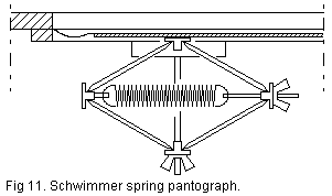
But there is a marvel called a bellows. Ideally a bellows can render an infinite capacitance, meaning the pressure is constant (DP =0) when you push in or take out a limited volume DV. - A concussion bellows is the standard decoupling device used to subdue pressure variations such as those we discuss here. There are two common forms, 'winkers' and 'schwimmers'. A winker is a small hinged bellows, often mounted in the wall of a trunk. It is pushed on by a compass spring to match the average pressure. You can fine adjust the point where the spring force is applied to a suitable distance from the hinge of the moving board.
A difficulty with concussion bellows is that you have to match the spring force quite precisely to the actual pressure. It is a passive device that adapts to the pressure, whatever this happens to be, it does not regulate it. If the spring force is too high or too low, then the bellows will stay in one of its end positions and will not be able to supply any volume displacements. With a schwimmer adjustable pantograph like in fig.11 you can adjust both the spring constant and the spring force operating on the plate. You can then come very close to infinite capacitance, i.e. constant pressure independent of plate position, but for this to be practical pressure must be closely regulated. Many organ chest designs, such as Aeolian, Pitman or WurliTzer, have the bottom of the chest occupied with various machinery, and there is no room for a schwimmer. These makers solved the problem differently, by placing another regulator close-coupled to the chest with a large opening. This essentially isolated the chest from any dynamic or pressure loss effects of the trunking. See Section 7 for an analysis of the entire wind supply configuration, including this feature. 5. Bellows speedAn issue with concussion bellows and regulators is how fast they react. In 3.2 the theme was about the effort to accelerate a mass of air inside a trunk. Now, about how difficult to accelerate the lid of a bellows. Again we can use the property of acoustical mass, and we can find (by way of how area relates force to pressure and speed to flow) an expression for the acoustical mass Ma of a bellows lid asMa = Mm/A2 [kg/m4]= [Ns2/m5] Acoustical mass of a pistonwhere Mm is the mechanical mass in kg and A is the lid area in m2. Intuition is strongly connected to mechanical mass (in kg or lb) - a heavy mass is hard to accelerate. However this does not directly apply when we look at the consequences for the air, then we must also account for the coupling area. The result of this is the acoustical mass - one may rephrase this into (pressure drop) per (flow increase rate) - admittedly difficult to understand by intuition, but it tells an important tale. Examples 8: Table relating mehanical mass and
area to acoustical mass. The first two items represent air in trunks. The
last three represent the lids for a small bellows and a big reservoir.
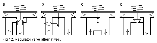
One might believe that 12 tiny grams of air in the 5 meter, 5 cm dia. tube should not do too much to slow down the air supply. But the resulting Ma says it indeed does so quite a lot! It is 25 times more difficult to accelerate the air in this trunk than it is to accelerate the small spring loaded bellows lid. So such a small bellows would do a lot of good as a compensator if you have that trunk. On the other hand, if you want it to maintain a sizable pressure using a weight instead of a spring, this weight would slow down the response of the bellows to make it good for nothing in the present circumstances. The last example underlines the significance of area. Despite an enormous amount of iron to accelerate it is very fast responding. Mostly valid: bigger is better. 6. RegulatorsThe purpose of a pressure regulator is to keep pressure at its output to be constant, whatever input pressure you supply and whatever flow load you demand. Any regulator has two main components: a sensor to monitor what is the actual output pressure, controlling an effector, some kind of valve that opens up just enough for the unregulated input. This can be implemented many ways, but here we limit ourselves to simple mechanical solutions, applicable to organs.A regulator may be characterized by its 'droop', telling how much pressure drops, DP, when you increase flow DU. The ratio between those two is then measured in [N/m2]/[m3/s] = [Ns/m5]. This is nothing else but acoustical impedance once again. Low droop and low (output) impedance is the same thing. Two factors decide this droop, or impedance. One is the sensor sensitivity. With our simple mechanically operating regulators the sensor is a spring and bellows. The spring compliance together with the bellows characteristic tell how far the bellows lid is displaced by any pressure change DP. The other factor is how big flow change DU is induced by the effecting valve when displaced this much. Next interesting property is the speed of regulation. This is where the preceding section 5 about bellows speed comes in, the acoustical mass (not its mechanical in kg) of the sensor bellows puts a limit to its reaction speed. An additional important feature with a regulator is its stability. Theoretically, the simple regulators considered here are mass-spring systems, so called first order, which should always be stable. But even within this narrow scope practical solutions are not always so, there may be additional elastic and inertial elements introducing extra delays and a more complicted higher order behavior. In particular the load can make for problems, it may for instance be another trunk where waves can propagate back and forth like in example 5 and present a complicated situation for the regulator. Also the wedging action of bellows ribs may cause a negative acoustical capacitance (meaning pressure goes down rather than up when you inject an air volume) which in itself is enough to trigger instability. Fig. 12 shows four regulator variants a - d. In all cases the unregulated input enters at the left side, and all have the same sensor element at the output, namely a bellows at top where the lid area and the spring force define what the regulated pressure is going to be. An essential feature for a good regulator, and for all these, is that the input unregulated pressure does not put any direct force on the sensor, neither any force to operate the valve - the output pressure should be independent of the input.. a has a sliding cylinder valve, the principle is the same as a knife valve regulator, common in player pianos. It may be difficult to make the slider with enough precision. If there is some play between it and the outer cylinder to ensure smooth running, then it will not be airtight enough when there is no load and the output pressure may rise beyond control. This can be somewhat repaired by making another hole in the output tube, bleeding it to atmosphere when the plunger goes up above the closed position. b is a variation using a "stove damper", "butterfly", or rotating disc as the inlet valve, the usual arrangement on the Spencer Orgoblo blower system so common on old American organs. In practice, the damper is weighted closed, and opened by a long chain through pulleys, from the top of the reservoir to the damper crank on the fan discharge. Crude, but effective if you accept the low speed caused by the weight. c with a rolling rubber cloth curtain against a grid is a quite good workaround to ease leakage problems. The soft curtain will rest tightly against its supporting grid and its actuating rod is easy to lead through a leather packing or just a small hole. This item is the same device as the sack reservoir in section 2. In all cases a-c the regulating valves have a relatively long mechanical travel between their fully open and closed positions. This impedes regulation accuracy but improves stability. d is a classical design, inspired from the Aeolian organ with Zeb Vance. Here the regulating valve is just a disk covering a hole, easy to make it airtight with a leather gasket. Its very essential distinctive feature is the small relief bellows below the disk. This one insures independence from the input pressure with the important proviso that its bellows cross sectional area must be about the same as the valve hole area. The valve disk requires a quite small displacement between open and closed positions. Speed of regulation accords with the acoustical mass of the lid and there are no critical friction elements. Indeed it may easily become too fast, meaning unstable. This is very conveniently damped by the viscous gas friction in the hole connecting the interior of the relief bellows to the ambient - in case of instability you can slow regulation down using a smaller hole. The area of the regulator valve opening should be perhaps twice the areas of the connecting trunks. Because the flow path is rather irregular in the valve region a small opening would give an unnecessary kinetic pressure drop in it when fully open. All the illustrated regulators are shown with a comparatively big bellows lid sensing the output regulated pressure. This is very deliberate. First reason is this enables the lid to exert a considerable force on the valve to overcome friction and other disturbances, this insures precision. Second, it automatically serves as a secondary reservoir/compensator. 7. Complete feeder systemsA complete feeder system is more complicated to analyze than the sum of its components, but some additional aspects can be illustrated with the scenario of fig. 13 - of course there are other ones possible. Top half is a schematic drawing of a source, a trunk, a regulator/concussion bellows, and finally the load in form of a chest. Below that is a circuit diagram of the same thing, it intentionally looks like an electrical one. This is the kind of thing you use in acoustics to compute what is happening. Such is nowadays done with network simulation computer programs, but classically it was simulated with such electrical analog circuits, using plain capacitors, inductors, and resistors.
#1. A 'distant' branch comprising the trunk, slowly reacting because of the inertia of the enclosed air mass. From the definition of acoustical mass we can estimate a characteristic time constant like in example 4 Dt=(Md*DU)/(Pr-Pc). A high acoustical mass Md for the trunk and a large flow increase DU will make it takes a long time Dt before supply stabilizes. You can shorten that time by widening the trunk (decreasing Md) or increasing the regulator margin Pr-Pc, the pressure difference between reservoir and chest. #2. A 'near' branch where the movement of the regulator bellows lid compliance Cr delivers the temporarily required extra puffs of air at transient loads, until the 'heavy' air in the trunk has had its time to accelerate. Its speed to do this is limited by the acoustical mass Mr of the lid, examples 8. To be efficient the lid acoustical mass must be appreciably smaller than that of the trunk. To be sufficient the lid area and displacement must be big enough to supply the flow during the transient time Dt. This can be translated into a rough estimate for necessary bellows displacement volume to be Vb=DU*Dt. #3. A 'fast' branch with the acoustic capacitance Cv of the local regulator bellows volume and other nearby volumes. This one delivers air immediately by virtue of its decompression, essentially without inertia, but has little capacity (!). V/(r*c2) is small with reasonable volumes, this amount of air is enough only for very short times. It is conventional good practice to have a large volume here, but this will hardly be sufficient anyway, recall example 7. When you stop the loading airflow, then the trunk flow carries on by
its inertia and rapidly fills up the regulator bellows such that its valve
closes abruptly. The trunk flow then suddenly 'hits the wall' and there
will be an appreciable pressure surge at the regulator input which can
be computed from Ztube and U, compare horror example
5. This underlines it is necessary the regulator valve be insensitive
to input pressure, otherwise it might not be capable of preventing this
surge to proceed into the regulated chest area.
8. References[1] From Audsley, G A: The Art of Organ-Building, (1905), Dover 1965, vol II, p 690, fig. CCCLXXVII[2] Carlsson, T.: On wind system dynamics of pipe organs. Lic. thesis, Chalmers Univ. of Technology, Göteborg 1999, fig. 18. [3] Finch, T. L., Nolle, A. W.: Pressure wave reflections in an organ note channel. J. Acoust. Soc. Am. 79(5), May 1986, pp 1584-1591. [4] Karlebo handbok. A different source is http://www.process-support.com/html/pressure_drop.html where you can enter arbitrary data and have the drop computed by a Java applet, provided you give the necessary parameters in SI units. These two sources render essentially the same results. [5] See e.g. http://www.laukhuff.de/english/ventus_e.html [6] See http://www.physics.nist.gov/Pubs/SP811/contents.html for a survey of SI units [7] Supplied by courtesy of Hans van Oost [8] By courtesy of Richard Z Vance 9. Unit conversions and Air propertiesUnit conversions
Air properties at atmospheric pressure and 20 deg C:
10. AcknowledgementRichard Z. Vance gave many valuable suggestions, improvements, and contributions in the process of reviewing this manuscript.Johan Liljencrants 2001-12-18 |
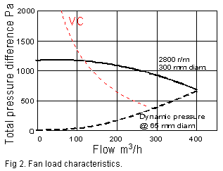 Fancy
drive alternatives from over the times are now displaced by ubiquitous
electric centrifugal fans. These have radically different properties from
a bellows, you can show them with a load characteristic graph. Fig.
2 is an example of such, how the output pressure can vary as function of
the flow delivered. The red dashed curve, where VC stands for a typical
vacuum cleaner fan, shows a very high pressure at low flow, dropping considerably
as load increases. This common fan type is about the least suitable there
is for an organ. But fans may be radically different from each other. By
proper engineering, including swept rotor blades, you can get a much superior
characteristic having almost constant pressure, as exemplified with the
black solid curve. The figures nearby show typical rotational speed (for
a 3 phase, 50 Hz motor) and diameter for a fan that can deliver pressures
in the 1 kPa (4 inWC) range. A fixed fan design delivers pressure in proportion
to radius and to the square of speed. For higher pressures you would normally
select a bigger fan (or possibly more than one in cascade) rather than
belt drive to a faster and noisier one.
Fancy
drive alternatives from over the times are now displaced by ubiquitous
electric centrifugal fans. These have radically different properties from
a bellows, you can show them with a load characteristic graph. Fig.
2 is an example of such, how the output pressure can vary as function of
the flow delivered. The red dashed curve, where VC stands for a typical
vacuum cleaner fan, shows a very high pressure at low flow, dropping considerably
as load increases. This common fan type is about the least suitable there
is for an organ. But fans may be radically different from each other. By
proper engineering, including swept rotor blades, you can get a much superior
characteristic having almost constant pressure, as exemplified with the
black solid curve. The figures nearby show typical rotational speed (for
a 3 phase, 50 Hz motor) and diameter for a fan that can deliver pressures
in the 1 kPa (4 inWC) range. A fixed fan design delivers pressure in proportion
to radius and to the square of speed. For higher pressures you would normally
select a bigger fan (or possibly more than one in cascade) rather than
belt drive to a faster and noisier one.
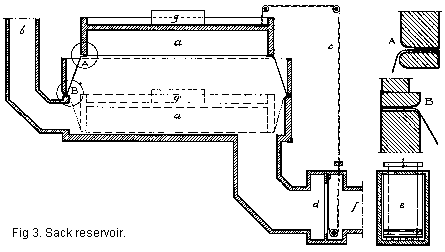 The
reservoir is conventionally a single wedge bellows or a double parallel
moving bellows (church organs). Another variant is the sack reservoir where
the lid is joined to the support frame with a rubber cloth collar that
rolls inside and out as the lid moves, fig. 3
The
reservoir is conventionally a single wedge bellows or a double parallel
moving bellows (church organs). Another variant is the sack reservoir where
the lid is joined to the support frame with a rubber cloth collar that
rolls inside and out as the lid moves, fig. 3 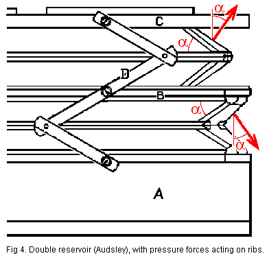 Fig.
4
Fig.
4
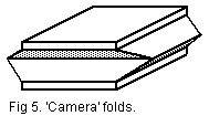 If
you make a square 'camera folded' bellows as in fig. 5 - cylindrical cloth,
two folds out, two in - this is also essentially neutral to the rib forces.
If
you make a square 'camera folded' bellows as in fig. 5 - cylindrical cloth,
two folds out, two in - this is also essentially neutral to the rib forces.
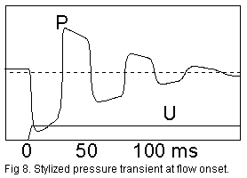 The
surge wave will continue for some time bouncing back and forth in the trunk
which actually behaves just like an organ pipe resonator. This idealized
fig. 8 shows pressure vs. time at the receiving end of the trunk.
The
surge wave will continue for some time bouncing back and forth in the trunk
which actually behaves just like an organ pipe resonator. This idealized
fig. 8 shows pressure vs. time at the receiving end of the trunk.
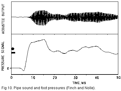
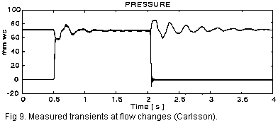 Here
are two illustrating examples taken from the real world. Recently Carlsson
Here
are two illustrating examples taken from the real world. Recently Carlsson
 In
a schwimmer the moving wall is a flat bellows cloth supporting a light
panel and this is often mounted in the wall of the pipe chest itself, the
ultimate location to avoid any ducting between compensator and point of
use.
In
a schwimmer the moving wall is a flat bellows cloth supporting a light
panel and this is often mounted in the wall of the pipe chest itself, the
ultimate location to avoid any ducting between compensator and point of
use.
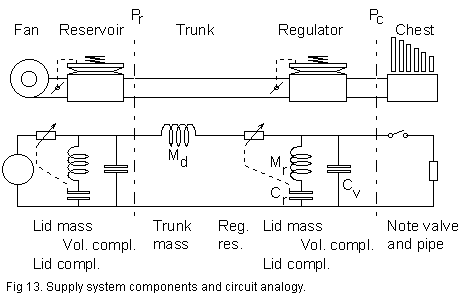 The
left basic supply, a feeder and reservoir, is supposed to deliver a constant
pressure
Pr whatever you load it with. To that end it
is normally a complete regulated system in itself, it has basically the
same elements and works the same way as the following regulation system.
With fan blowers it is common that the first regulating valve (controlled
by the reservoir lid) alternatively is put at the fan intake rather than
at its outlet. Then follows a trunk, the problem child, leading to the
wind chest where pressure is Pc. The trunk causes temporary
pressure drops and surges at changes in the load. To close or open the
switch in the electrical diagram corresponds to start or stop playing pipes.
From the circuit diagram we may describe the middle supply regulator system,
between Pr and Pc, to have three branches,
there are three different ways for flow to arrive at the note valve switch:
The
left basic supply, a feeder and reservoir, is supposed to deliver a constant
pressure
Pr whatever you load it with. To that end it
is normally a complete regulated system in itself, it has basically the
same elements and works the same way as the following regulation system.
With fan blowers it is common that the first regulating valve (controlled
by the reservoir lid) alternatively is put at the fan intake rather than
at its outlet. Then follows a trunk, the problem child, leading to the
wind chest where pressure is Pc. The trunk causes temporary
pressure drops and surges at changes in the load. To close or open the
switch in the electrical diagram corresponds to start or stop playing pipes.
From the circuit diagram we may describe the middle supply regulator system,
between Pr and Pc, to have three branches,
there are three different ways for flow to arrive at the note valve switch:
|
|
|
|
|
|
|
|
|
CONTACT FORM: Click HERE to write to the editor, or to post a message about Mechanical Musical Instruments to the MMD Unless otherwise noted, all opinions are those of the individual authors and may not represent those of the editors. Compilation copyright 1995-2026 by Jody Kravitz. Please read our Republication Policy before copying information from or creating links to this web site. Click HERE to contact the webmaster regarding problems with the website. |
|
|
||||||
|